Introduction
Visual effects companies have a long history of struggling for solvency, but the dramatic bankruptcies of Digital Domain and Rhythm & Hues in 2012 and 2013 have brought the VFX industry’s business model into public debate.
Without getting into issues of tax subsidies and cheap overseas labor, I wanted to explore ways that a profitable company could still be put out of business by an unpredictable and unforgiving market, and perhaps even be surprised by it.
I began by looking at cash flow. What is the impact of a volatile market and tight margins? What if a company didn’t manage their cash correctly? A few bad months could quickly eat through cash reserves and make it very difficult to recover fast enough to stop the damage.
In an attempt to understand how cash flow can affect a profitable company in an unpredictable industry I developed a simple model to demonstrate the effects of volatility. Based on Stanford Professor Sam Savage’s work (see Acknowledgements, below) I created a simulation in Excel that takes expenses, profit margin, starting balance, growth rate, and market volatility as inputs. The spreadsheet calculates monthly expenses and revenues for ten years under five thousand different random scenarios. The results are analyzed to show a probable range of outcomes.
An important disclaimer: I have no unique visibility into R&H or DD’s businesses. These numbers are not related to either of their financials, and are certainly very far off from those particular situations. I am not trying to specifically model either of those businesses. This is simply an exploration of business models, inspired by the current status of the VFX industry.
Volatility
The primary driver of this simulation is volatility – a number that approximates how unpredictable the revenue stream is. With zero volatility, monthly revenue is equal to expenses plus the profit margin (we’ll ignore growth for the moment). As volatility increases, revenue becomes less predictable, varying randomly within a range but maintaining the same average.
The revenue is based on a random walk model, where over time the average is predictable, but the value for any particular point in time is not. In my model a volatility of 50% represents a market where at any given month the company’s revenue can be as low as zero or higher than twice the expenses plus profit margin. This is far from an exact representation of any industry, but I felt it reflected the extremes of what may happen to a VFX company – they may be fully booked one month and have no work the next, and under special circumstances they may be able work at an extremely high profit margin for a brief burst of time (known as “911” work). The beauty of building a model is that we can experiment with different assumptions for volatility. More details about the math are given at the end of this post if you are interested.
First Examples
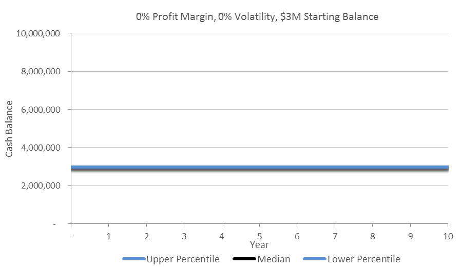
We will start with very simple assumptions to explain the model, and then work up to some interesting conclusions. The first example assumes a stable company with zero growth, $1M in monthly expenses and $3M of cash in the bank (a safety net of three months of operating expenses). With zero profit margin and zero volatility, the company will break even each month and always have $3M in the bank.
A chart of cash in the bank each month for ten years is flat and boring.
We can now add volatility into the model by randomizing the revenue within a range each month. Over a long enough period of time this revenue will average $1M per month, but in any given month can be a healthy profit or loss. By running the simulation thousands of times and analyzing the results we can get a statistical approximation of the outcome. The model runs 5,000 different ten year scenarios and allows us to see a view of probabilities of what could happen to a company in this situation.
Keeping everything else the same and increasing volatility to 50% gives us this result:
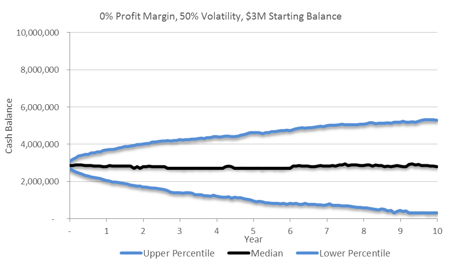
The black median line is a type of average outcome – it represents a 50/50 probability that a company’s results could be higher or lower. Not surprisingly, this corresponds to revenue with zero volatility. The lines above and below the median show the 33rd and 67th percentiles in either direction – in other words, 33% of the 5,000 simulations fall below this range and 33% are over it.
The Gambler’s Ruin
If you relied on this simulation to design your business model you’d be in trouble, though, because it doesn’t tell the whole story. There is no bankruptcy scenario yet – we have allowed our companies to have unlimited debt. The model doesn’t yet show how many of the companies hit insolvency somewhere along the way, which would have caused them to fold up shop.
![]()
We can simulate bankruptcy by adding a condition to the spreadsheet where if a company’s cash balance goes below zero then it stays at zero from then on.
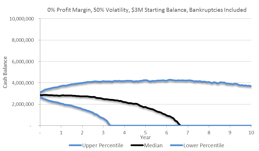
Suddenly the picture looks quite bleak. By year three almost a third of the companies have gone out of business and by year seven more than half are bankrupt.
What we learn is that most of the companies had streaks where they used up their $3M reserve – it could have been three devastating months in a row, but much more likely it was a long stretch of small losses mixed with occasional wins.
If there is one lesson in this whole exercise, this is it. Like the Gambler’s Ruin, without deep enough pockets you will eventually lose to the house. To mitigate this, you need to tilt the odds in your favor.
Profit Margin
In the case of our companies, tilting the odds means increasing the profit margin. The model allows us to do this, and we find a 4% margin is the magic point where the median company survives, and possibly even prospers, long term.

In this scenario 70% of the companies survive to ten years, and over 50% of all companies grow their cash reserves, giving them even more protection against volatility. In fact, they can start investing some of their cash in growing their company.
Growth
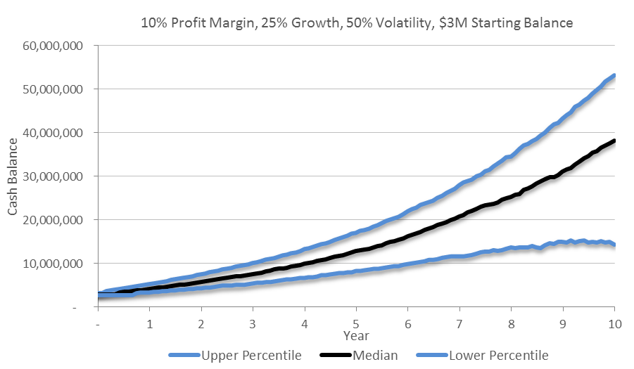
If we wanted to grow our $12M/yr revenue company to $100M/yr we would need to grow at 25% per year for ten years – not an unreasonable rate. With the meager 4% profit margin, the company would likely be out of business within 5 ½ years, with less than a 30% chance of surviving to year ten. Under this very simple model, increasing the profit margin to 10% gives the company a reasonable chance of getting there.
Conclusions
This model shows the impact of a single dynamic – volatility – in what is actually a very complex market. There are a myriad of other factors that affect a real business’ cash flow like payment terms, defaulted or delayed payments, access to outside financing or short term loans, etc. Nonetheless, it is important to learn that companies need a positive profit margin to survive in a volatile market. That positive margin allows for extra cash reserves to be built up in order to carry the company through down cycles.
There are three things a company can do to protect itself from the dangers of an unpredictable market.
- Lower the volatility, or in portfolio theory terms: diversify. This does not mean offer more products and services to the same six clients, it means work for different clients in markets that are not on the same business cycle.
- Increase profits. Don’t grow for the sake of growth, and certainly don’t expand into lower margin businesses. Higher revenue with a lower margin increases the risk dramatically.
- Conserve cash. A larger cash reserve allows the company to survive more dry periods, but it doesn’t tilt the odds in the company’s favor in the long term, only profits do that.
Acknowledgments
Dr. Savage inspired me to build this model after I read his book, “The Flaw of Averages.” He also spent quite a few hours re-educating me about statistics and coaching me on tools he’s made available at ProbabilityManagement.org. Thanks, Sam.
The Model
Stop reading unless you’re really curious about how the model works!
I used SIPMath, a set of Excel macros from ProbabilityManagement.org, to build the model quickly and much more efficiently than I could do by hand. The model begins with a monthly expense of $1M times a growth rate for 120 months. Monthly revenue is that expense amount times a profit margin. Very simple so far.
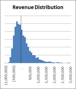
Through the magic of the macros, the model is put through 5,000 trials with the revenue for each month of each trial being changed randomly according to the volatility. The random numbers follow a log normal distribution. Log normal was suggested as the best way to model financial numbers lacking any real data – its distribution has a mean of 1 and it never goes below 0, and many real world markets follow a similar distribution. For our case of 50% volatility, the revenue distribution (pre-growth or profit margin) looks like this:
I also tried the model with a straight random distribution and a normal distribution. The same conclusions would have been reached with any of them, but the log normal behaved the best. The model would support real world data, and an interesting next step would be to get anonymous data from the industry to use for the revenue distribution.
You can download the 16MB file here: CashFlowModelDist5000LogN on Dropbox. It needs Excel 2010 or newer to run. It is also a machine hog – each time a variable is changed it does over 620,000 calculations, so expect to wait a few seconds between updates. The sheet titled “Dashboard” has all the variables you can tweak plus the charts.